HelixMC Tutorial
| Release: | 0.9 |
|---|---|
| Date: | May 13, 2016 |
This tutorial demonstrates how to install and run simple calculations with HelixMC, and breifly summarizes available examples and bp-step paramerter database. For details on the classes and functions availble, please see HelixMC Reference.
Install
Currently HelixMC has only been tested on Linux. It should run on other Unix-like system (e.g. Mac OS X). The following packages are also required by HelixMC. The versions we used are given in parathesis.
- Python (2.7.3)
- Numpy (1.6.1)
- Matplotlib (1.1.0)
- A working C/C++ compiler. Here we used GCC (4.6.3)
The easiest way to setup the python environment is to use latest Enthought Python Distribution (http://www.enthought.com/).
The easiest way to install is to use pip install:
$ pip install helixmc
Alternatively, one can download the source code from the latest GitHub repository. Simply run:
$ git clone https://github.com/fcchou/HelixMC.git
Or you can go to https://github.com/fcchou/HelixMC/ and download the source code by clicking the “Download ZIP” button.
After this, you can instal HelixMC using setup.py:
$ python setup.py build
$ sudo python setup.py install
Instead of installing using setup.py, you can just add your HelixMC folder
into the system’s $PATH and $PYTHONPATH. In bash this can be done by
adding the following lines to your ~/.bashrc:
export PATH=$PATH:<HelixMC Path>
export PYTHONPATH=$PYTHONPATH:<HelixMC Path>
Then build the Cython extension. Under the helixmc/ folder, run:
$ python _cython_build.py build_ext --inplace
Note that this requires you to have Cython installed. Otherwise you can choose to build the c source file, then you do not need Cython:
$ python _c_build.py build_ext --inplace
Now you should be all set. To test the install, simply run:
$ helixmc-run --help
This should output the help information for helixmc-run application.
Run HelixMC
The helixmc-run application wraps the classes and functions of HelixMC to allow simple MC job submissions from command line.
A detailed help for all options of helixmc-run can be obtained
by running:
$ helixmc-run --help
Now we demonstrate a simple example for helixmc-run.
First, run the following command to kick out a MC run:
$ helixmc-run -params DNA_default.npz -n_bp 100 -n_step 10 -seq GCCG \
-force 5 -compute_fuller_link -out_frame test_run
Here, -params give the input database file that contains bp-step
parameters curated from PDB (by default it searches the helixmc database folder
if it does not find the input file). -n_bp is the total number of bp in the
helix. -n_step is the number of MC steps. -seq gives the sequence of
the nucleic acids (ATCG for DNA and AUCG for RNA). -force is the applied
z-direction stretching force. -compute_fuller_link tells HelixMC to compute
and store the linking number using Fuller’s approximation [R1].
-out_frame option will make HelixMC save the final frame to disk as
test_run.npz in this case.
Depending on your machine it will take a few seconds to run. After completion you should see something like:
Total time = 1.941772
Accept rate = 0.787879
It is advisable to check the Accept rate of each run, and make sure it is not too low. As a rule of thumb, if Accept rate < 0.1, this means most MC moves are rejected, and you will need use a higher-than-normal number of MC steps to acheive the same level of sampling.
Now we can analyze the output data. Open a Python session and enters the following:
>>> import numpy as np
>>> from helixmc.pose import HelixPose
The observables for each frame are stored in MC_data.npz. Normally the
coordinates and reference frames of the last bp are recorded. If
-compute_fuller_link or -compute_exact_link is used, the twist and
writhe of the helix will also be stored (note that link = twist + writhe).
For example I can compute the average z-extension and the average link as follows:
>>> data = np.load('MC_data.npz')
>>> data.files
['coord_terminal', 'twist', 'writhe', 'frame_terminal']
>>> data['coord_terminal'][:,2]  # 2 for the z-elements
array([ 309.06198311,  317.92717085,  320.17158221,  304.42561971,
        319.07461907,  306.94162915,  314.7566295 ,  319.04106375,
        322.42125203,  325.72718993])
>>> np.average(data['coord_terminal'][:,2])  # avg. z-extension in Å
315.95487393228649
>>> np.average(data['twist'] + data['writhe'])  # avg. link in radian
60.648749666780688
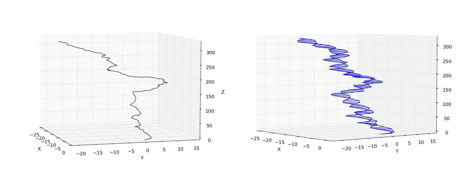
Remember we stored the final frame of the simulation to test_run.npz. We
will now plot the helix using that:
>>> pose = HelixPose('test_run.npz')
>>> pose.plot_centerline()  # plot the centerline
>>> pose.plot_helix()  # plot the entire helix
You should see something similar to the following
This is the end of the example. For more examples, check the examples/
folder in HelixMC, which is briefly summarized below.
Other Examples
Here is a list of examples in the examples/ folder.
| force_ext: | This is just the example above. |
|---|---|
| link_cst: | This is for link-contrained simulation, similar to the torsioal-trap single-molecule experiment [R2]. |
| z-dna: | Simulation of Z-DNA using helixmc-run. |
| fuller_check: | Check the if the Fuller’s approximation is correct in certain criteria. |
| data_fitting: | How to use helixmc.fitfxn to fit simulation or experiment
data to simple analytical models. |
| helixplot: | More examples for plotting the helices. |
| lp_olson: | How to perform alternative evaluation of bending persistence length using the method suggested by Olson et al. [R3]. |
| bp_database: | Examples on curating bp-step parameters from PDB. |
Base-pair Step Parameters Database
In the helixmc/data/ folder, several different bp-step parameter sets are
given. These datasets were all extracted from structures in Protein Data Bank
(PDB, http://www.pdb.org/), with different selection and filtering. The list
below summarizes these data.
| DNA_default: | B-DNA data from structures with resolution (Rs) <= 2.8 Å, excluding protein-binding models. |
|---|---|
| DNA_2.8_all: | A-DNA + B-DNA, Rs <= 2.8 Å, including protein-binding models. |
| DNA_2.0_noprot: | B-DNA, Rs <= 2.0 Å, excluding protein-binding models. |
| RNA_default: | RNA, Rs <= 2.8 Å, excluding protein-binding models. |
| RNA_2.8_all: | RNA, Rs <= 2.8 Å, including protein-binding models. |
| RNA_2.0_noprot: | RNA, Rs <= 2.0 Å, excluding protein-binding models. |
| Z-DNA: | Z-DNA, Rs <= 2.8 Å, including protein-binding models. |
| *unfiltered: | Unfiltered datasets (no filtering of histogram outliers). |
| DNA_gau: | Single 6D Gaussian built from DNA_default. |
| RNA_gau: | Single 6D Gaussian built from RNA_default. |
| DNA_gau_graft: | Chimera dataset with mean from DNA_gau and covariance from RNA_gau. |
| RNA_gau_graft: | Chimera dataset with mean from RNA_gau and covariance from DNA_gau. |
| *gau_refit: | Manually refitted datasets to match experimental measurements. |
| *_2.8_all_?bp: | Multi-bp datasets derived from the 2.8_all pdb lists. |
Note that Gaussian dataset (*gau*.npy) must be loaded with
-gaussian_params tag in helixmc-run command line (instead of
-params). Also Gaussian dataset does not support sequence specific
simulations.
The corresponding lists of PDB models being used are given in the
helixmc/data/pdb_list/ folder.
These datasets are in npy/npz format (Numpy array/archive). For the npz files,
the data for different bp-steps of different sequences were separated into
different arrays in the file. For B-DNA and RNA, parameter sets with
Rise >= 5.5 Å or Twist <= 5° were thrown away as outliers. Then, parameter
sets with values beyond 4 standard deviations away from the mean for any
of the 6 bp-step parameters were also removed. For B-DNA (except
DNA_2.8_all, where the protein binding makes A-DNA and B-DNA
unseparable), we further clustered the data using k-means algorithm to
separate the A-DNA and B-DNA data. Note that these filtering steps are
skipped in the unfiltered datasets.
For Z-DNA, we only considered two types of bp-steps: CG and GC. We used the following selection criteria: Twist <= -30° for GC, and -30° < Twist <= 5° for CG. For CG bp-steps, we further filtered the data by only keeping parameter sets with 4.5 Å <= Rise < 6.3 Å. Parameter sets with values beyond 4 standard deviation away from the mean were then removed, similar to the above cases.
See also examples/bp_database/ for a detailed example for the
curation of DNA_2.0_noprot.npz.
References
| [R1] | Fuller FB (1978) Decomposition of the linking number of a closed ribbon: A problem from molecular biology. PNAS 75: 3557-3561. |
| [R2] | Lipfert J, Kerssemakers JWJ, Jager T, Dekker NH (2010) Magnetic torque tweezers: measuring torsional stiffness in DNA and RecA-DNA filaments. Nature Methods 7: 977–980. |
| [R3] | Olson WK, Colasanti AV, Czapla L, Zheng G (2008) Insights into the Sequence-Dependent Macromolecular Properties of DNA from Base-Pair Level Modeling. In: Voth GA, editor. Coarse-Graining of Condensed Phase and Biomolecular Systems: CRC Press. pp. 205-223. |